
Power, minimal detectable effect, and bucket size estimation in A/B tests
By
Tuesday, 8 March 2016
Bucket size estimation for A/B experiments
In previous posts, we discussed how to detect potentially biased experiments, and explored the implications of using multiple control groups. This post describes how Twitter’s A/B testing framework, DDG, addresses one of the most common questions we hear from experimenters, product managers, and engineers: how many users do we need to sample in order to run an informative experiment?
From a statistical standpoint, the larger the buckets, the better. If all we cared about was how reliably and quickly we could observe a change, we would run all tests at a 50/50 split, which is not always advisable. New features have risk, and we want to limit risk exposure. Also, if experimental treatments change as we iterate on designs and approaches, we might confuse a lot of users.
Additionally, if all experiments ran at a 50/50 split, our users could wind up in multiple experiments simultaneously, making it difficult to reason what anyone should be experiencing at any given time. Thus, if 1% of the traffic is sufficient to measure effect of changes, we would prefer to use only 1%. However, if we pick too small a bucket, we might not be able to observe a real change, which will affect our decision-making and/or slow down iteration while we re-run the experiment with larger buckets.
To address this problem, we created a special tool to provide guidance for experimenters on sizing their experiment appropriately, and to alert them when experiments are likely to be underpowered.
Prior art
There are many different experiment sizing and power calculation tools available online. They tend to either explicitly ask the experimenter the sample mean and standard deviation (in addition to overall population size) or they address “click through rate” (CTR) or “conversion” — binary-valued metrics (either 1 or 0) for which variance is easy to calculate given the ratio of 1s to 0s.
None of these were straightforward to incorporate into our experiment creation workflow, for two reasons:
A quick review of statistical power
Let’s first define a few terms.
Null hypothesis is the hypothesis that the treatment has no effect. An A/B test seeks to measures a statistic for control and treatment, and calculates the probability that the difference would be as extreme as the observed difference under the null hypothesis.
This probability is called the p-value. We reject the null hypothesis if p-value is very low. The conventional threshold for rejecting the null hypothesis is 5%.
Power is the probability that an experiment will flag a real change as statistically significant. The convention is to require 80% power. Power depends on magnitude of the change, and variance among samples.
True effect is the actual difference of mean between the buckets that would have been observed if we had infinitely large sample sizes. It’s a fixed but unknown parameter, which we are trying to infer. The difference we compute from the samples is called the observed effect and is an estimate of the true effect. Given sample size and sample variance, we can calculate the smallest real effect size which we would be able to detect at 80% power. This value is called the minimal detectable effect with 80% power, or 0.8 MDE.
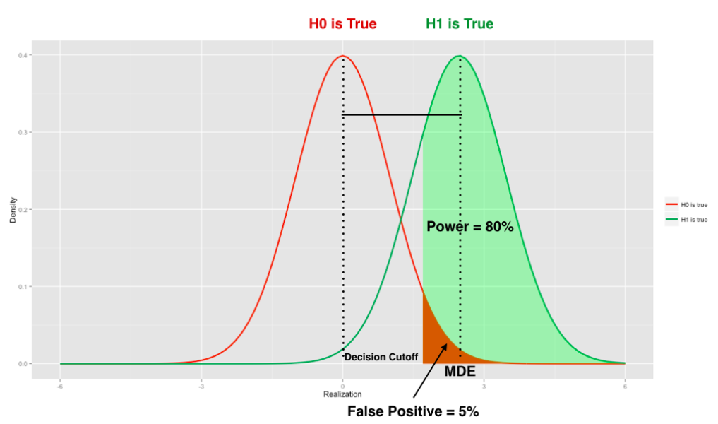
The graph below — which applies to a one-sided two sample t-test — helps us visualize all this. The two bell-shaped curves represent the sampling distribution of the standardized mean difference, under the null hypothesis (red) and the alternative (green) respectively.
The umber-colored area illustrates false positives — the 5% chance of getting a measurement under the null hypothesis that is so far from the mean that we call it statistically significant. The green area illustrates the 80% of time we call statistical significance under the alternative. Note there’s a lot of red and green to the left of the MDE — it is possible to observe a statistically significant change that is less than “minimal detectable effect” under the conventional cutoff values of 0.05 p-value and 0.8 MDE (you can’t observe it as often as 4 out of 5 times, but you can still happen to observe it).
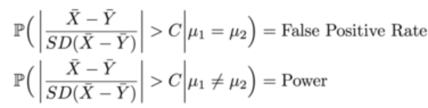
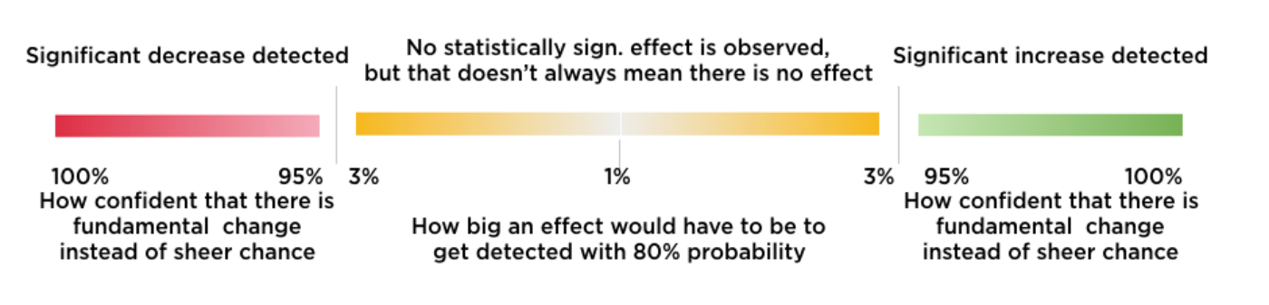
We can represent false positive rate and power (of a two-sided test) in the following way:
As experimenters, we want to increase our power and decrease the false positive rate. Low statistical power means we can miss a positive change and dismiss an experiment that would have made a difference. It also means we can miss a negative change, and pass through as harmless an experiment that in fact hurts our metrics.
Ensuring we can get sufficient power is a critical step in experiment design.
Sizing an experiment
There is one big lever we can use to get desired power: the bucket size. We want to allocate enough traffic that we can detect the effect, but not so much that we’re practically shipping the feature. To figure out how large our bucket sizes need to be, let’s take another look at the power formula. Assuming a false positive rate of 5% and a two-tailed test, we see that power can be represented by:
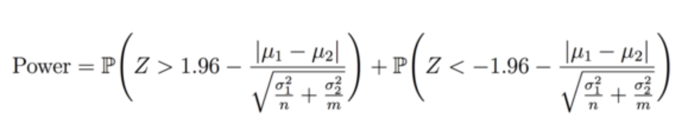
Here, Z is the distribution of the standardized mean difference. The difference of mus is the true effect size, and sigmas represent the standard deviation of the metrics in control and treatment buckets, respectively. Sizes of each bucket are represented by n and m. Finally, 1.96 is the C from above when we set false positive rate to 5% (the curious can find derivation in any statistics textbook).
Given this equation, we can make a few assertions on how to increase power:
If we use the convention of requiring power to be at least 80%, and make the simplifying assumptions that we have equal bucket sizes (n = m) and that the sigmas are the same, we can derive a nice formula for sample size n, as a function of true effect size and variance (via Kohavi et al [1]).
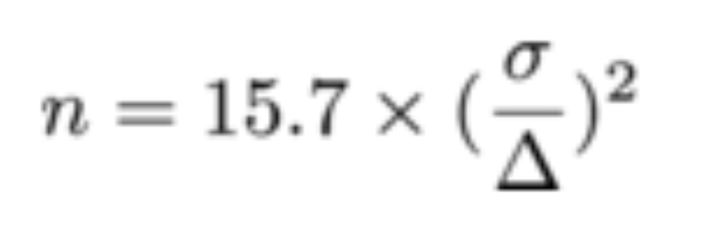
With this simplified formula in place, we need to get a handle on delta and sigma — the true effect size and standard deviation, respectively.
Bucket size estimation tool
Since we can’t rely on collecting metric variance or standard deviation for the specific sampled populations directly from the experimenters, we created a tool that can make suggestions based on basic data the experimenter can get more easily.
The key insight is that while in theory, an experiment can be instrumented anywhere in the app, many product teams at Twitter tend to instrument experiments in relatively few decision points. Stable products also tend to reuse their custom metrics between experiments. In these cases, we have a rich set of experiment records and historical data that we can use to estimate the sigmas for an upcoming but similar experiment. Our tool simply asks the experimenter to provide an ID of a similar experiment from the past, and loads up observed statistics from that experiment for all metrics the experiment tracked. The experimenter can now choose any of the previously tracked metrics, specify how much of a lift they expect to see with new changes, and get accurate estimates on the amount of traffic they need to allocate to reliably observe the expected change.
In cases where no prior experiments have been instrumented in the same location, or when brand new metrics are necessary, an experiment can be started in “dry-run” mode, just bucketing into control. The regular experiment pipeline will collect all the statistics necessary for buckets to be estimated.
Calling attention to underpowered metrics
Sometimes the bucket estimation tool isn’t enough. Experimenters may discover that their experiment targets an audience with different behavior from the audience of the experiment they provided for bucket size estimation. They may also want to assess impact on metrics that were not taken into account when using the bucket estimation tool. In such cases, it’s possible that a given metric has insufficient power to make a strong claim regarding experiment results. We call attention to metrics for which no significant effect is detected, and the minimal detectable effect is large.
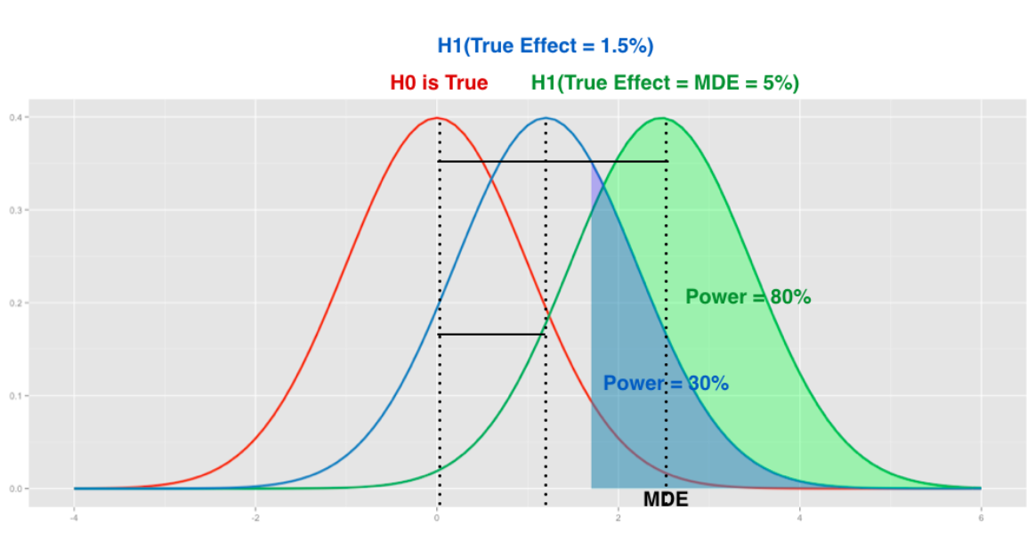
Consider a hypothetical experiment that attempts to improve the “Who To Follow” suggestion algorithm. Let’s imagine that historical experiments of this sort tend to produce a gain of 1% more follows. In the current experiment, we measure a 1.5% observed effect but it isn’t statistically significant. We also calculate that based on the current sample size, MDE is 5%.
Based on past experience, we know that if there is a true effect, it’s unlikely to be above 5%. With the MDE we measured, it’s unlikely we would call a “real” 1.5% change statistically significant. In fact, the graph below demonstrates that only 30% of experiments of this size would detect a 1.5% change as statistically significant. Considering the high MDE, instead of concluding that the proposed improvement has no effect, it’s better to increase the sample size and re-run the experiment with higher power.
The Twitter experimentation framework, DDG, provides visual feedback to experimenters by coloring statistically significant positive changes green, and statistically significant negative changes red. We color likely-underpowered metrics a shade of yellow. The intensity of the color is used to call experimenters’ attention to the actual p-values when we see statistical significance, and to potential power problems when we do not. The intensity of red and green colors depends on the p-value (the more intense, the lower the p-value). The intensity of the yellow depends on the MDE (the more intense, the higher the MDE).
Summary
Providing the right amount of traffic is critical for successful experimentation. Too little traffic, and the experimenter does not have enough information to make a decision. Too much traffic, and you expose a lot of users to a treatment that might not fully ship. Power analysis is a critical tool for determining how much traffic is required. DDG uses data collected from past experiments to guide experimenters in selecting optimal bucket sizes. Furthermore, DDG provides visual feedback to help experimenters detect whether their experiments are underpowered, allowing them to rerun with larger sample sizes if needed. If your A/B testing tool does not have similar capabilities, there’s a decent chance you are missing “real” changes due to being underpowered — both good changes that improve your product, and bad effects that are affecting you negatively. Call your data scientist today, and ask them about power analysis.
Acknowledgements
Robert Chang and Dmitriy Ryaboy co-authored this blog post.
[1] R. Kohavi, R. Longbotham, D. Sommerfield, and R. M. Henne. Controlled experiments on the web: Survey and practical guide. Data Mining and Knowledge Discovery, 18, no. 1:140–181, July 2008.
Did someone say … cookies?
X and its partners use cookies to provide you with a better, safer and
faster service and to support our business. Some cookies are necessary to use
our services, improve our services, and make sure they work properly.
Show more about your choices.