Distributed training of sparse ML models — Part 1: Network bottlenecks

At Twitter, we use machine learning (ML) models in many applications, from ad selection, to abuse detection, to content recommendations and beyond. We're constantly looking to improve our models, try out new ideas, and keep our models up to date with the freshest data possible. This depends on our ability to train and retrain those models quickly.

Model training is a process where a large amount of data is analyzed to find patterns in the data. In a trained model, those patterns are encoded into a complex network of parameterized functions, which can guess the value of a missing piece of information. Many of our models are trained on sparse data, meaning that the data has a lot of fields but only some are populated with values.

In our efforts to increase our developer velocity and have more relevant models, we have sought to scale this up through distributed model training in TensorFlow. The issue, however, is that these sparse models don't distribute well with standard TensorFlow, mostly due to network bandwidth limits.

Using customized distributed training, we increased the performance by 100X over the standard TensorFlow distribution strategies. This also gave us a 60X speedup for the same workload compared to training on a single machine. This allows us to iterate faster and train models on more and fresher data.

In this first of three posts (Parts 2 and 3 on optimization strategies and training speedups, respectively), we detail the main ideas and optimizations behind these changes. Let's begin by diving into the distribution strategies provided by TensorFlow, and the difficulties we had using them.

The basic parallelization strategies

There are two common strategies for parallelization of model training: data parallelism and model parallelism.

Data parallelism

In machine learning, the data we work with is a series of examples that contain a sample and a label. A sample is a collection of features, which are the individual field values. Each sample is paired with a label that describes the desired output of the model. With enough of these examples, a model learns how to guess an appropriate label when provided with an unlabeled sample. The parameters of a model are the values that control its decision making. These are updated by applying small changes to the values through a process called stochastic gradient descent. This entire process is known as model training.

In the simplest scenario, this update process involves stepping the parameters in the direction that most quickly improves the model output. Pseudocode for this update looks like the following:

Machine learning algorithms work a little backwards. We think of things in terms of loss, which is something we want to minimize. In this algorithm, the function `model_loss_grad()` tells us the direction to change the model parameters that most quickly makes the model output worse. We identify this direction, and step in the opposite direction.

We can make model training more parallelizable by making updates to `params` using small batches of data, each sample computed in parallel and summed before applying. This technique is called data parallelism, and can be summarized as follows:

Data batching can allow for parallelism both in a single machine through multithreading, as well as in distributed training through such training methods as TensorFlow’s parameter server strategy and AllReduce.

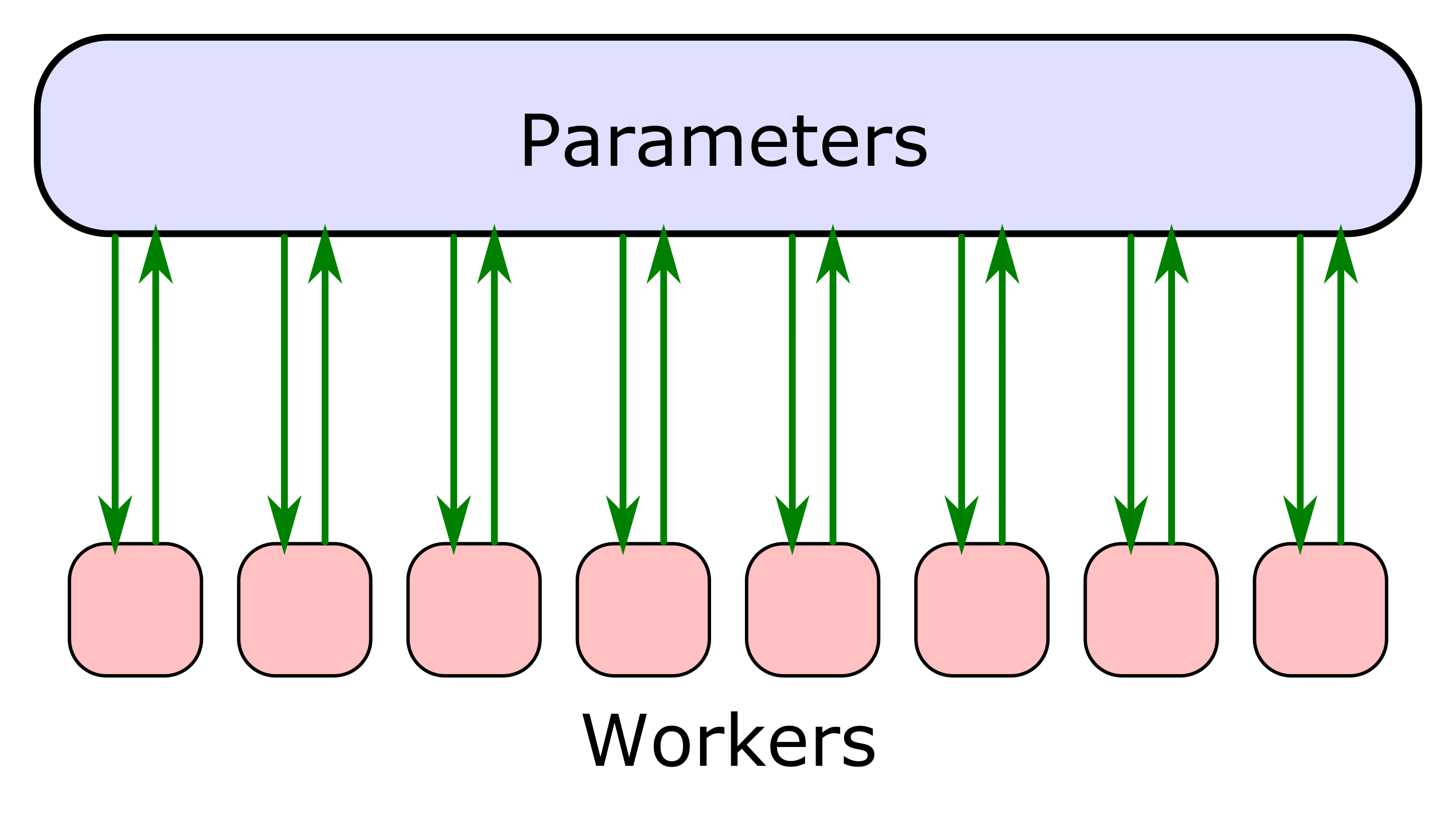
The ordering of the batches is often not significant to the quality of the results, so the algorithm can be parallelized further by allowing asynchronous updates, where workers independently compute mini-batches of gradients based on whatever view of the model parameters they happen to have at the start of their iteration. This is depicted in Figure 1.1.

Model parallelism 

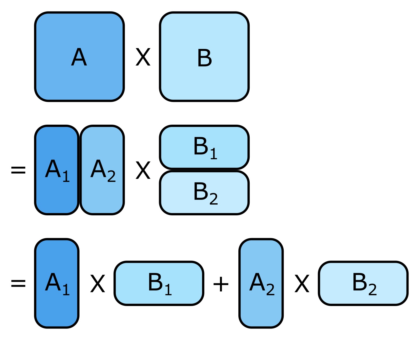
Model parallelism is the other fundamental way of parallelizing a model. In this type of parallelism, the model intrinsically has sub-computations that can be broken down into parallelizable chunks. For example, matrix multiplication and other linear algebraic operations can often be partitioned and parallelized. This kind of parallelization tends to require specific tailoring to the given model, but model parallelism can help improve performance in both multithreaded single-node training as well as distributed (multinode) training scenarios.

Matrix multiplication is an example operation where we can use model parallelism. It can be split up into parallel calculations, as shown in Figure 1.2.

Unfortunately, these two forms of parallelism — data parallelism and model parallelism — have not worked well for distributed training of the kind of models that are prevalent at Twitter. In the following sections, we provide details on the special characteristics of these models and why we cannot simply use these basic parallelization techniques.

Sparse models — a common model type at Twitter

Many models at Twitter operate on data with a large number of input fields — potentially hundreds of thousands — but for any given example, only a few hundred of these features are actually present. This is called sparse data, which is in contrast to dense data that typically has a much smaller number of mostly nonzero entries. Models that use sparse data come with particular challenges that we explain below.

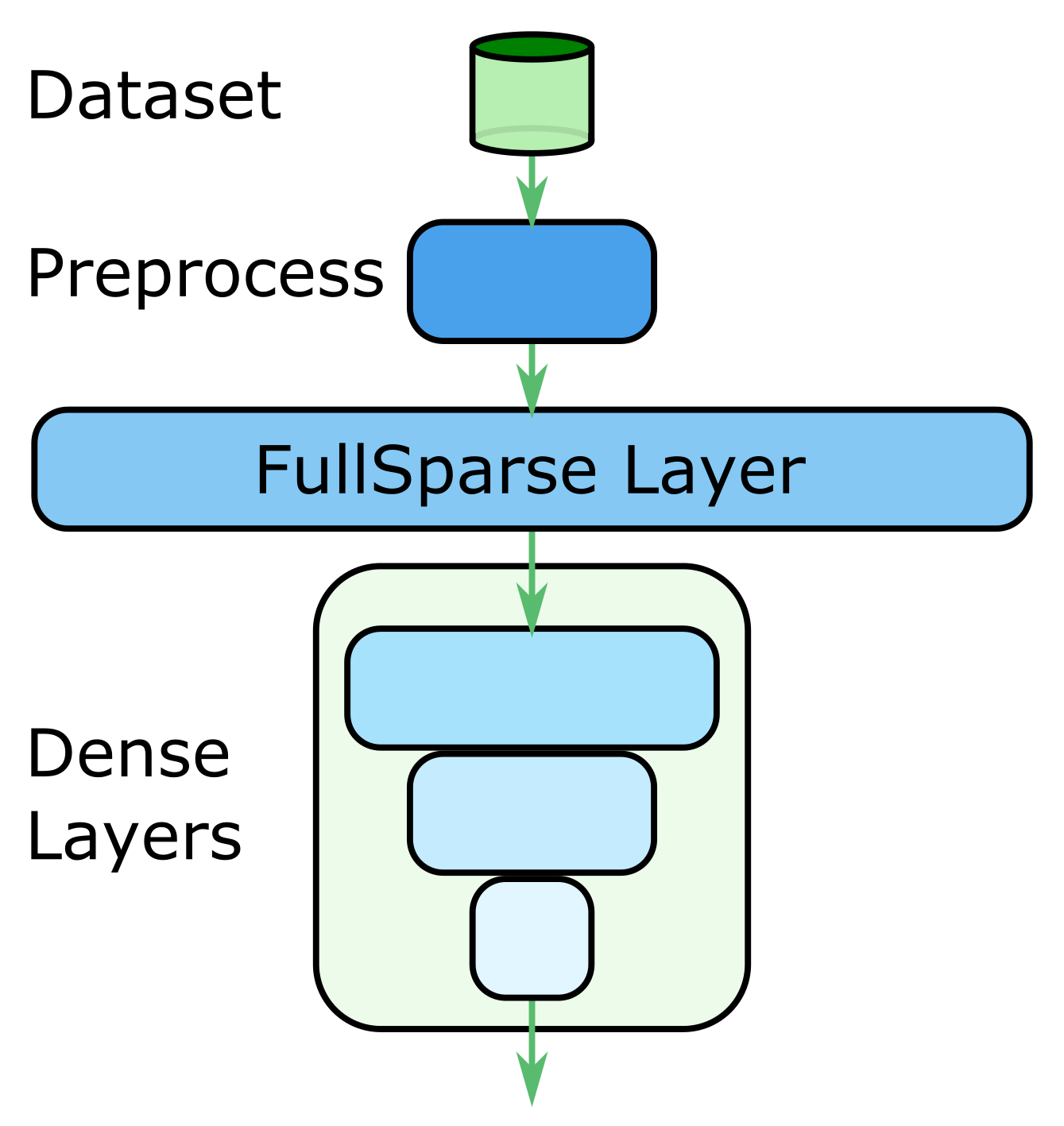
In deep learning, models are composed of layers of parameters with connections between them. Most of the time the layers are fully connected, which means that all the inputs of a layer are connected to each of its outputs. Typically, we feed this sparse input to a fully connected layer, which we call a FullSparse layer. Output from the FullSparse layer might then go to a number of typically much smaller fully connected dense-input layers.

Such a model is shown in Figure 1.3. Here, we first pull data from a dataset. We then do some decoding and preprocessing of the data to produce the sparse input data. This sparse input then goes to the FullSparse layer, which produces a dense result. Often, our models also have some number of additional fully connected layers, which then produce the final model output. It is also possible to have more complicated models that have multiple sparse inputs and additional dense inputs. In these cases, we would have a separate FullSparse layer for each of the sparse inputs.

Examples of such an architecture include ads split net and the timelines Tweet ranking model. Both of these actually have multiple FullSparse layers, due to the input samples being split into a number of separate input feature groups.

The problem

Our machine learning models are typically large — up to 2GB in size. Our FullSparse layers usually have an input size of 2^18 to 2^22 with an output size of around 50 to 400. This leads to sparse layer sizes of 100MB to 1GB, or more. The potential for multiple sparse layers in combination with the parameters of the rest of the model adds up to models of significant size.

Our data centers have multiple services running side by side. Since the network is a shared resource, there are egress (transmit) and ingress (receive) limits to prevent any one service from consuming too much bandwidth and starving the others.

Our egress limits have been in the 100MB to 1000MB per second range. This results in a significant performance bottleneck. Transferring the parameters and gradients between components is prohibitively slow in a standard distributed TensorFlow setup.

Let’s look more closely at distributed training in TensorFlow. TensorFlow supports distributed training through data parallelism in a number of ways.

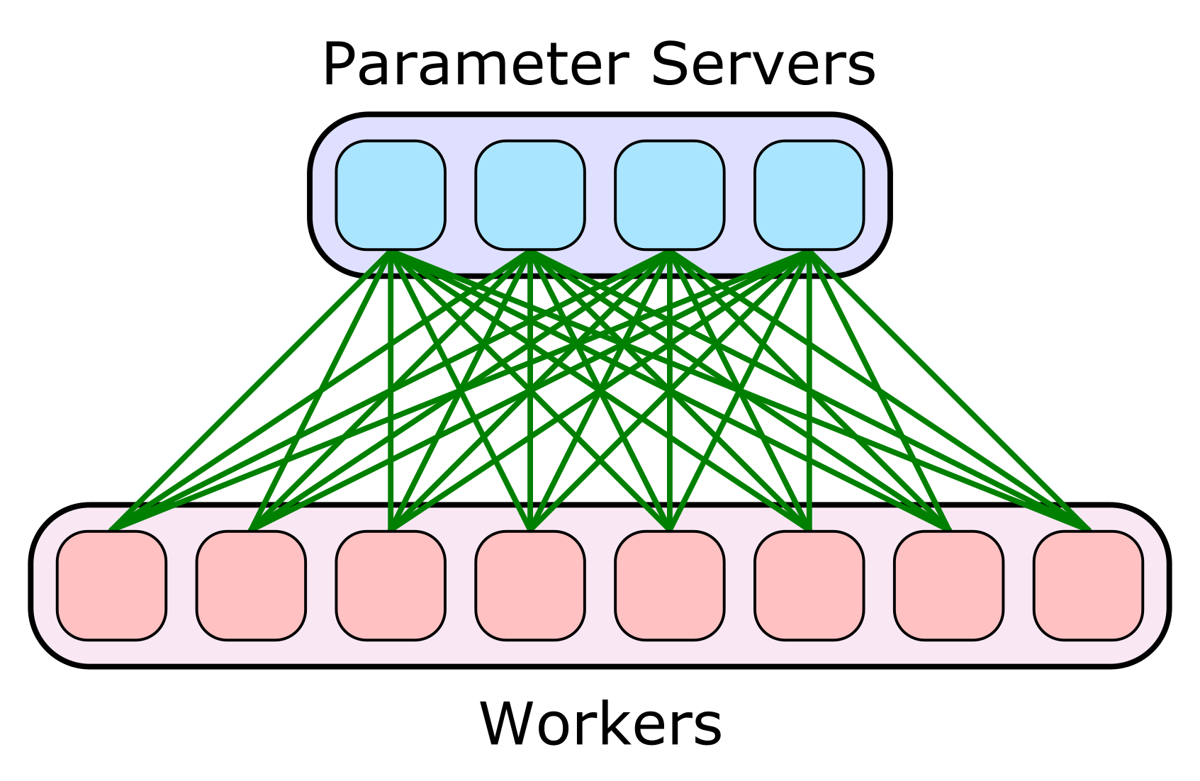
First, let's consider the Parameter Server (PS) distribution strategy, as seen in Figure 1.4. In TensorFlow, this includes both ParameterServerStrategy and CentralStorageStrategy. Under this strategy, the majority of computations happen in worker nodes, while the parameters of the model are kept in separate nodes called parameter servers. A worker needs to have both the parameters and the data to compute an update for the parameters. All the parameters must be sent from the parameter server to the worker and then the results sent back at the end. If a model has 1GB of parameter data, this can be very costly, as that is sent twice.

When we focus on the transfer of parameters in this strategy, we get the following best-case steps per second, in terms of the network limits and model size:

In this description, `NumPS` is the number of parameter servers and `egress` is the transmit rate limit for the parameter servers. This optimistic estimate takes into account only the time to transmit parameters from the parameter servers to a worker, and ignores computation time, ingress limits, transmission time of parameter updates, and other factors that contribute to decreased training speed. Specifically, this speed limit is the maximum frequency at which we can send the full set of model parameters over the network from the parameter servers to a worker.

A simple example shows that this theoretical limit is unacceptably slow. Consider a distributed training setup with 10 parameter servers, egress of 150MB/s, and model size of 2000MB. This results in steps per second less than 0.75, which corresponds with the actual training speed we see in a standard PS distribution strategy for our sparse models. Even with 10X the transmit bandwidth, we would get a maximum of 7.5 steps per second. We are able to train at much faster rates in a single-machine setup — typically tens of steps per second with optimal settings. This shows that the model size and network limits are killing this distribution strategy.

TensorFlow also supports distributed gradient descent algorithms based on AllReduce algorithms, including MirroredStrategy, TPUStrategy, and MultiWorkerMirroredStrategy. As with the PS strategy, the network limits result in unacceptable training speed for large models.

These issues with the standard TensorFlow distribution strategies force us to take a customized approach to distributed training that works better for our models, which we detail in Part 2, on optimized strategies.