Distributed training of sparse ML models — Part 2: Optimized strategies

In Part 1, on network bottleneck issues, we discussed the sparse models that are common at Twitter and the difficulties in using standard TensorFlow distributed-training strategies that arise from large sparse-model sizes and low caps on network speed.

In the second of three posts in the series, we show a custom approach to distributed training that takes into account the particular properties of sparse models.

The solution

We combine several techniques to get distributed training to work. These techniques use both model parallelism of the FullSparse layers and data parallelism to improve how the speed-limited network is used. We will build on our techniques one at a time to get an overall picture of how our distributed-training system works for sparse models.

Never transmit FullSparse weights

The first technique is to never send FullSparse weights or their gradients between nodes in the distributed-training cluster. As we have seen in the analysis of the parameter server and all-reduce strategies in the previous post, sending these weights or gradients with low data rates incurs a time-cost that is far too high. What this means is that whenever a computation involves weights of the FullSparse layer, that computation must be performed in the machine that is holding those weights.

Model parallelism — partition the FullSparse matrix multiplication

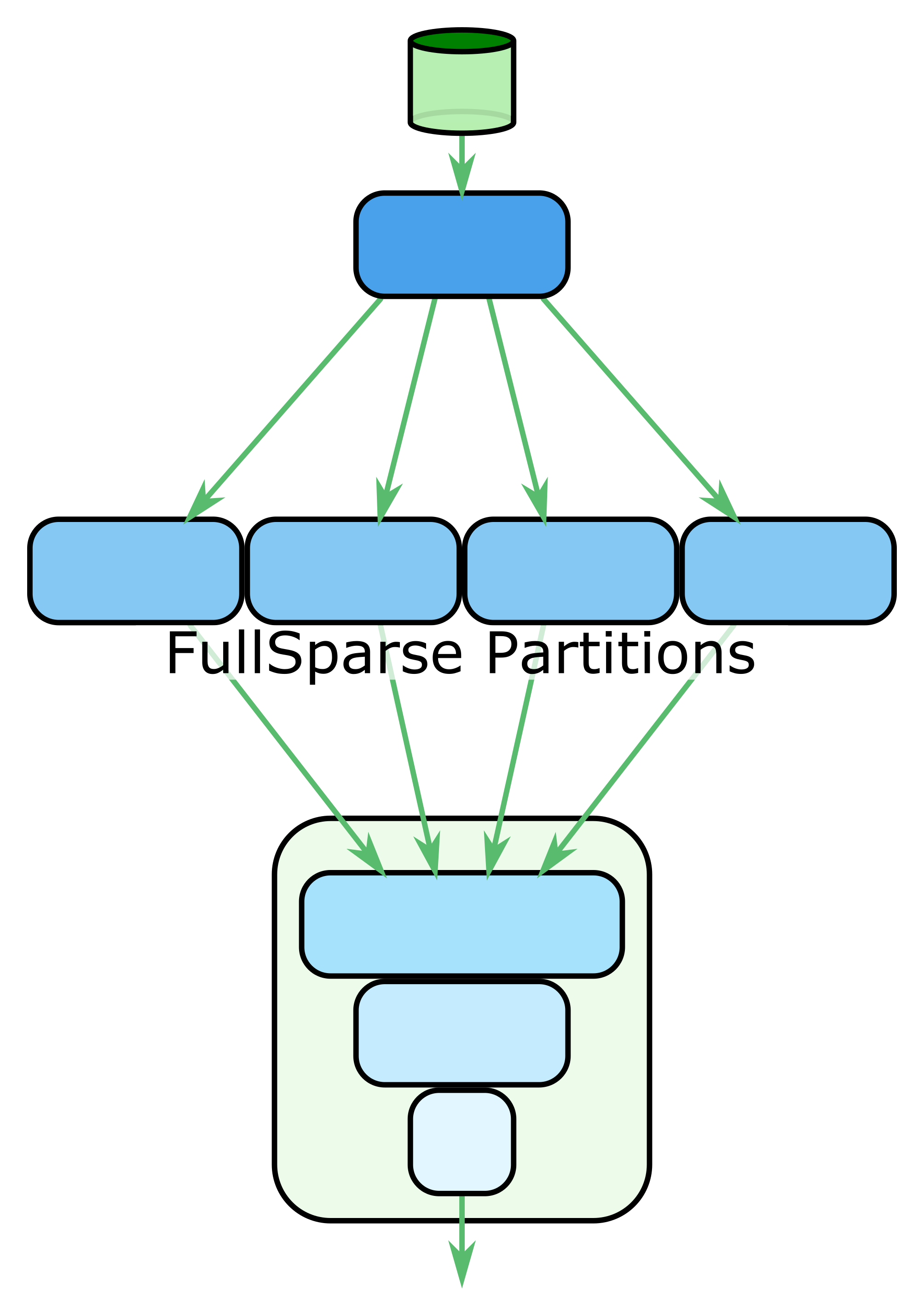
When examining the results of single-node performance profiling of our sparse models, we typically observe that the FullSparse layer computation takes a large portion of the total time to compute each model update. In fact, the bulk of this computation is a matrix multiply between the sparse input batch and the weights of the FullSparse layer. A natural way to parallelize these computations is to partition this matrix multiplication and use model parallelism. This is shown in Figure 2.1.

In this figure, we first retrieve and preprocess the data. Then we send it to the partitions of the FullSparse layer, and the results of the partition calculations are aggregated for the rest of the processing. Since we are trying to utilize a cluster of nodes distributed on a network, each of the FullSparse partitions will be in a separate node. Each of these nodes will both hold the weights for its assigned partition and perform any computations and updates that involve that partition of the weights. This removes the need to ever transmit those weights across the network.

Partition the weights on axis 0

To speed up data transmissions over the network, we want to further reduce the amount of data transmitted. The two simplest ways of partitioning the weights matrix of the FullSparse layer are along axis 0 (vertical) and along axis 1 (horizontal), and these affect how much data must be transmitted.

The matrix multiply in the FullSparse layer can be written as

where `X` is the input batch, one row per training sample, and `W` is the matrix of FullSparse parameters. We can partition `W` along axis 1 to get

Then the matrix multiply is the concatenation of the partitioned multiplies, as follows:

If we used this partitioning, the node for partition `j` would compute X·W_j and therefore would require the full data matrix `X` to be sent from the preprocessing node. In aggregate, the preprocessing node would send an amount of data equal to `P` times the size of the input batch for each model update.

If we instead partition on axis 0, we will have

We also need the input batch to be partitioned in this partition scheme, such that

Basically, we have partitioned the matrices into groups of features. The resulting matrix multiply is then

In this case, the node for partition `j` would compute X_j·W_j and therefore would require only a subset of the data matrix `X` to be sent from the preprocessing node. In aggregate, the preprocessing node would send an amount of data equal to the size of the input batch, which is better than what we previously found for axis-1 partitioning.

Data parallelism — asynchronous parallel batch processing

Simply using model parallelism of the FullSparse layer and partitioning along axis 0 is not sufficient for us to get the training speed gains we need. This is because the transmission of data from the preprocessing node to the nodes handling the FullSparse partitions still bottlenecks training speed, even with axis-0 partitioning.

Let’s consider the size of a typical training batch. For our sparse models, we can think of this sparse matrix as being represented by three lists — one for the row indices of each non-zero element, one for the column indices, and one for the values. In TensorFlow, the indices are represented as int64 integers, and the values are represented as float32 values. As such, there are 20 bytes for every non-zero element in the input batch. Typical training examples have around 1000 non-zero elements, so with an input batch of size 512 examples, that gives us batches of 1000 * 20B * 512 ≈ 10MB per batch. With egress limits of 150MB/s, we can only transmit and hence compute at most 15 batches per second in this model-parallel design. This is still too slow.

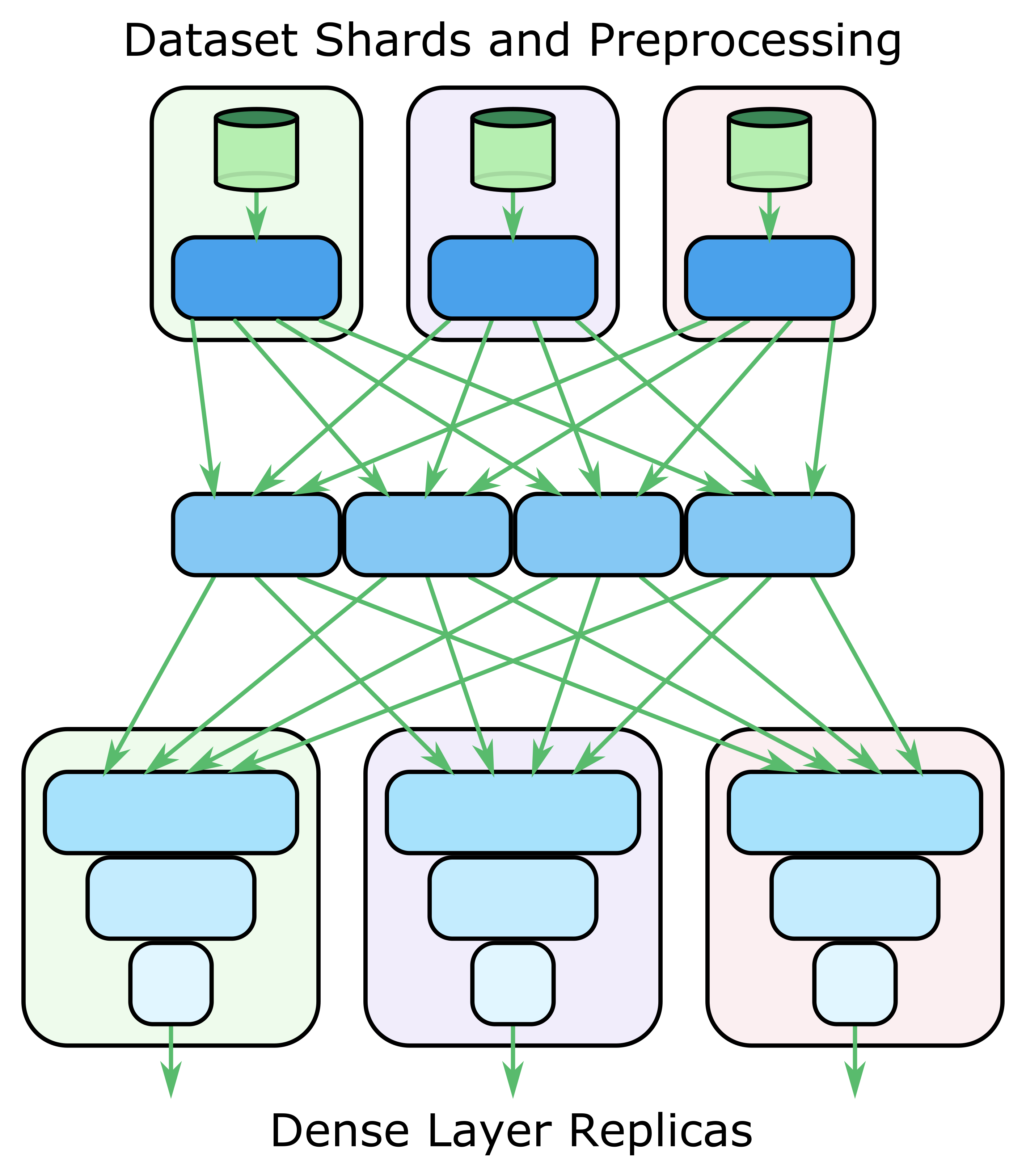
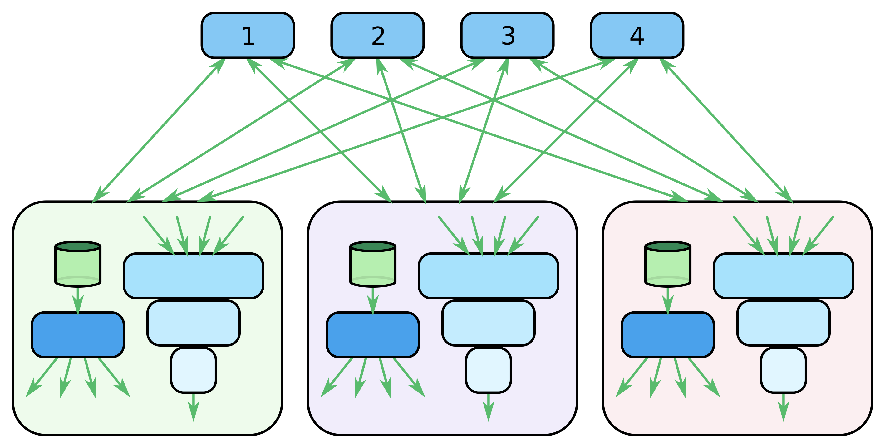
To overcome this bottleneck in transmitting the input batch, we use multiple input pipelines, as shown at the top of Figure 2.2.

Here we show several nodes that pull in different batches of data in parallel. These nodes do the preprocessing, split up the batches, and then send the data pieces to the FullSparse partitions. Once the components of the FullSparse are computed, they are aggregated again according to the original input batching. This prepares the batches for the computation of the rest of the model shown at the bottom of the figure (for example, the computation of the fully connected dense-input layers). In this way, the amount of input data ingested by the training system is able to scale up to meet the demand of the nodes handling the FullSparse partitions.

Placement of variables and operations

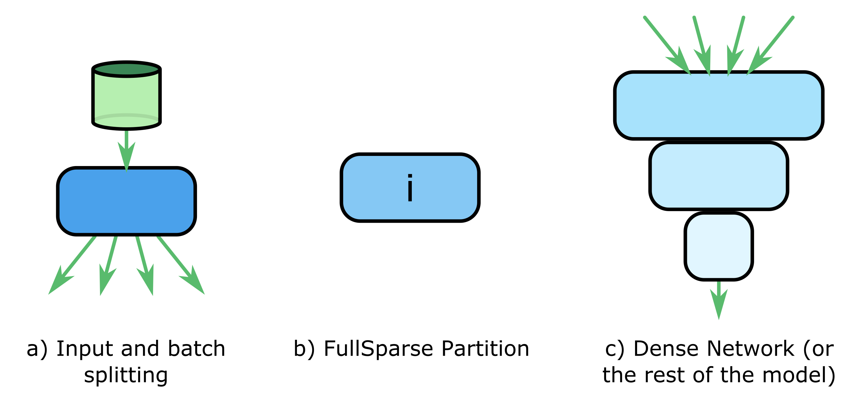
At this point, we have shown three basic components (Figure 2.3) of our distributed model, each of which will be associated with particular nodes in the training cluster:

• Input data pipeline and batch splitting
• FullSparse layer partitions and associated computations (including forward pass and backpropagation)
• Aggregation of FullSparse partition results and the rest of the model (including forward pass and backpropagation)

Note that there are other model variables not mentioned in the above three components, such as the subsequent fully connected layers after the FullSparse results are aggregated. However, it is assumed that these model variables are small enough in size that they can reside distributed in the cluster and be accessed with sufficient speed that they do not bottleneck training speed.

The question now is “How should we actually design the training cluster?” Our goal here is to choose the number of nodes in the cluster, assign potentially multiple functions to each of these nodes, and decide on an efficient allocation of resources.

An initial approach could be to directly allocate nodes for each of the components as shown in Figure 2.2. However, although the nodes in charge of the FullSparse partitions can remain busy by asynchronously receiving input batches, these are the only nodes that could maintain a constant workload. In one training step, the nodes in charge of the input pipeline will only be active up to the point that they transmit the partitioned input batch. Similarly, the nodes in charge of the layers after the FullSparse will only be active in the time between receiving the FullSparse results and sending back gradient information during backpropagation.

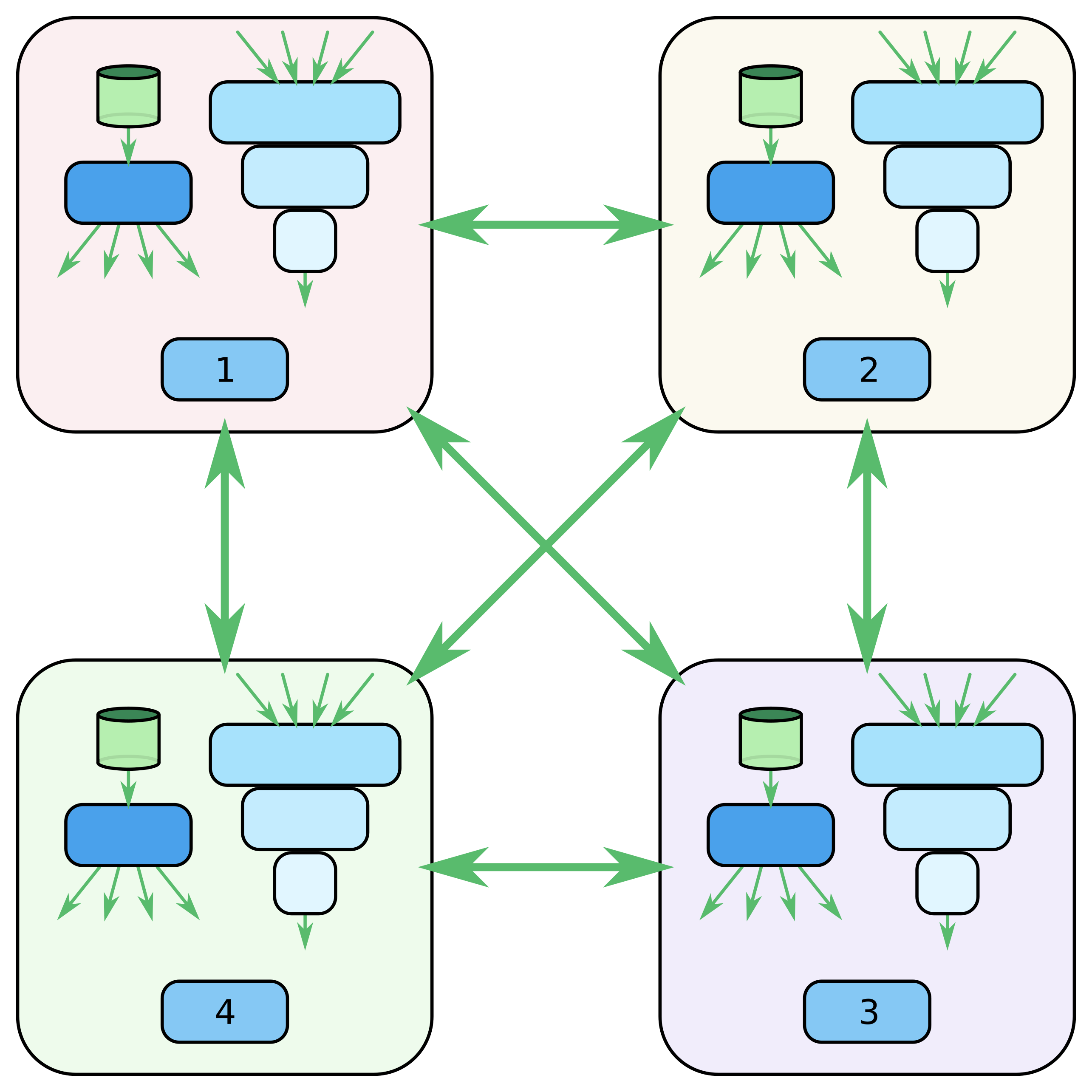
An alternative design that improves on the efficiency of this initial approach is shown in Figure 2.4, which we will call the Fully Connected architecture.

In this cluster topology, we use as many nodes as we have partitions of the FullSparse layer. (We also have a small number of parameter servers for maintaining the other model variables, which are not shown in the figure.) Each node is then responsible for a separate complete input pipeline, a single partition of the FullSparse layer, and a replica of the model layers that follow the FullSparse. This architecture allows all of the nodes to remain busy by either processing an input batch, updating the dense-input layers, or performing computations and updates for the assigned FullSparse partition.

Scaling up this architecture is simple — we just need to use more identical nodes and partition the FullSparse layer into smaller pieces. This works well because both the network-bandwidth requirements per node are independent of the number of nodes in the network, due to the axis-0 partitioning. Unfortunately, this architecture might have reliability issues. This is because each of these nodes contains a portion of the FullSparse weights. Nodes are stateful, so when a node is lost, the state must be recovered. In TensorFlow, we simply restore all of the graph variables from the most recent checkpoint. However, this results in some lost training time, due to the checkpoint not being fully up to date and the startup time for the replacement node.

A design that takes into account this reliability issue is shown in Figure 2.5, which we call the Bipartite architecture. This is the design we have settled on for widespread use.

Here, the FullSparse partitions are separate in their own training servers. In TensorFlow, these will be parameter servers, even though they are also assigned a significant portion of the overall computational workload. By making this separation, the nodes in charge of the input pipelines and the non-FullSparse parts of the model (the TensorFlow “worker” nodes) can remain stateless. This results in a setup where training can continue even when one or more of these worker nodes has been lost and needs to be restarted. Compared to other designs we have tried, this reduces the number of stateful nodes in the cluster with equivalent training throughput, which decreases the likelihood of needing to recover from the loss of a stateful node. Note that in this design, we have the issue that worker nodes may still sit idle while waiting for FullSparse results. However, in practice we have seen that we achieve comparable or even better performance to other designs for similar resource allocation.

Conclusion

Using the techniques described above, which combine aspects of both data and model parallelism, we significantly reduce the amount of communication required between distributed-training nodes. This significantly increases the throughput of our training cluster. In out third and final post in the series — on training speedups — we demonstrate the performance gains observed on real models used at Twitter.