Deep learning on dynamic graphs

Many real-world problems involving networks of transactions, social interactions, and engagements are dynamic and can be modeled as graphs where nodes and edges appear over time. In this post, we describe Temporal Graph Networks, a generic framework for deep learning on dynamic graphs. 

Background

Graph neural networks (GNNs) research has surged to become one of the hottest topics in machine learning this year. GNNs have seen a series of recent successes in problems from the fields of biology, chemistry, social science, physics, and many others. So far, GNN models have been primarily developed for static graphs that do not change over time. However, many interesting real-world graphs are dynamic and evolve over time, with prominent examples including social networks, financial transactions, and recommender systems. In many cases, it is the dynamic behavior of such systems that conveys important insights, which are otherwise lost if one only considers a static graph.

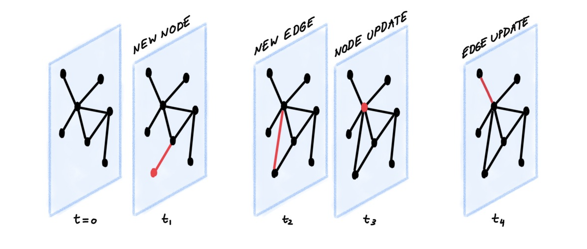
A dynamic graph can be represented as an ordered list or an asynchronous stream of timed events, such as additions or deletions of nodes and edges¹. A social network like Twitter is a good illustration: when a person joins the platform, a new node is created. When they follow another person, a follow edge is created. When they change their profile, the node is updated.

This stream of events is ingested by an encoder neural network that produces a time-dependent embedding for each node of the graph. The embedding can then be fed into a decoder that is designed for a specific task. One example task is predicting future interactions by trying to answer the question: What is the probability of having an edge between two nodes i and j at time t? The ability to answer this question is crucial to recommender systems that e.g. suggest to social network users who to follow or decide which content to display. Figure 3 illustrates this scenario:

In the example shown in Figure 3, TGN computes embeddings for nodes 2 and 4 at time t₈. These embeddings are then concatenated and fed into a decoder (eg. an MLP), which outputs the probability of the interaction happening.

The key piece in the above setup is the encoder that can be trained with any decoder. In the example task of future interaction prediction, training can be done in a self-supervised manner: during each epoch, the encoder processes the events in chronological order, and predicts the next interaction based on the previous ones².

Temporal Graph Networks

The Temporal Graph Network (TGN) is a general encoder architecture proposed in our paper with Fabrizio Frasca, Davide Eynard, Ben Chamberlain, and Federico Monti from Twitter. This model can be applied to various problems of learning on dynamic graphs. A TGN encoder has the following components:  

Memory.  The memory stores the states of all the nodes, acting as a compressed representation of the node’s past interactions. It is analogous to the hidden state of a recurrent neural network (RNN); however, here we have a separate state vector sᵢ(t) for each node i at time t. When a new node appears, we add a corresponding state initialized as a vector of zeros. Moreover, since the memory for each node is just a state vector (and not a parameter), it can also be updated at test time when the model ingests new interactions. 

Message Function. The message function is the main mechanism of updating the memory. Given an interaction between nodes i and j at time t, the message function computes two messages (one for i and one for j) , which are vectors used to update the memory. This is similar to the messages computed in message-passing graph neural networks (MPNNs)³. The message is a function of the memory of nodes i and j at the instance of time t⁻ preceding the interaction, the interaction time t, and the edge features⁴:

Memory Updater. The memory updater is used to update the memory with the new messages. This module is usually implemented as an RNN:

Given that the memory of a node is a vector updated over time, the most straightforward approach is to use it directly as the node embedding. In practice, however, this is a bad idea due to the staleness problem: since the memory is only updated when a node is involved in an interaction, a long period of inactivity causes the node’s memory to go out of date. 

As an example, imagine a person staying off Twitter for a few months. When they return they might have developed new interests in the meantime, so the memory of their past activity is no longer relevant. We therefore need a better way to compute the embeddings. 

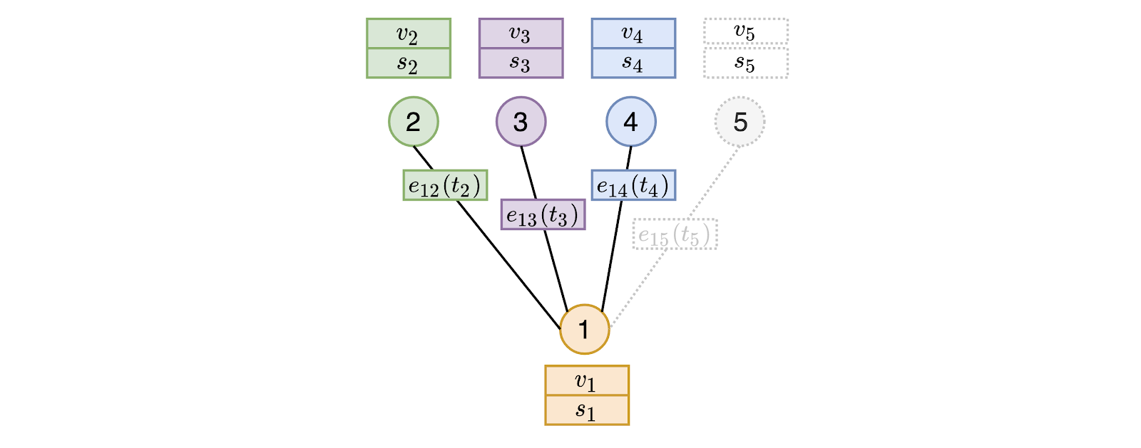
Embedding. A solution is to look at the node neighbors. To solve the staleness problem, the embedding module computes the temporal embedding of a node by performing a graph aggregation over the spatio-temporal neighbors of that node. Even if the node has been inactive for a while, it is likely that some of its neighbors have been active. By aggregating their memories, TGN can compute an up-to-date embedding for the node. 

In our example, even when a person stays off Twitter, their friends continue to be active, so when they return, the recent activity of their friends is likely to be more relevant than the person's own history.

In the above diagram (Figure 6), when computing the embedding for node 1 at some time t greater than t₂, t₃ and t₄, but smaller than t₅, the temporal neighborhood will include only edges occurred before time t. The edge with node 5 is not involved in the computation, because it happens in the future. Instead, the embedding module aggregates from both the features (v) and memory (s) of neighbors 2, 3 and 4, as well as the features on the edges to compute a representation for node 1. The best performing graph embedding module in our experiments is graph attention, which is able to learn which neighbors are the most important based on their memory, features and time of interaction. 

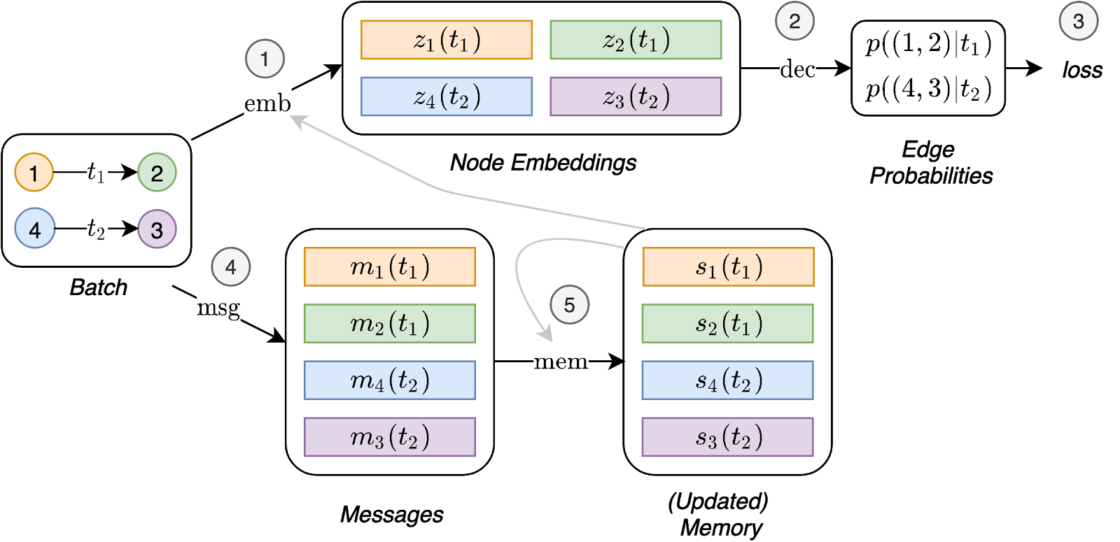
The computations performed by TGN on a batch of training data are summarised in the following figure:

Figure 7 shows that, on the one side, embeddings are produced by the embedding module using the temporal graph and the node’s memory (1). The embeddings are then used to predict the batch interactions and compute the loss (2, 3). On the other side, these same interactions are used to update the memory (4, 5).

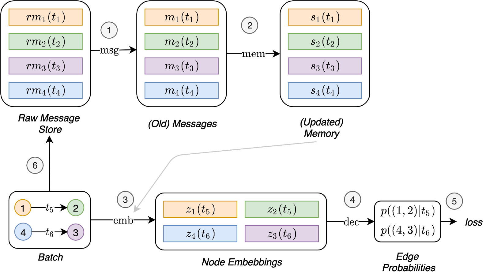
Looking at the above diagram, you may be wondering how the memory-related modules (Message function, Message aggregator, and Memory updater) are trained, given that they do not seem to directly influence the loss and therefore do not receive a gradient. In order for these modules to influence the loss, we need to update the memory before predicting the batch interactions. However, that would cause leakage, since the memory would already contain information about what we are trying to predict. The strategy we propose to get around this problem is to update the memory with messages coming from previous batches, and then predict the interactions. The diagram below (Figure 8) shows the flow of operations of TGN, which is necessary to train the memory-related modules:

Figure 8 introduces a new component, the Raw Message Store. Raw messages are the necessary information to compute messages, for interactions which have been processed by the model in the past. This allows the model to delay the memory update brought by an interaction to later batches. 

At first, the memory is updated using messages computed from raw messages stored in previous batches (1 and 2). The embeddings can then be computed using the just updated memory (grey link) (3). By doing this, the computation of the memory-related modules directly influences the loss (4, 5), and they receive a gradient. Finally, the raw messages for this batch interactions are stored in the raw message store (6) to be used in future batches.

Performance of TGNs

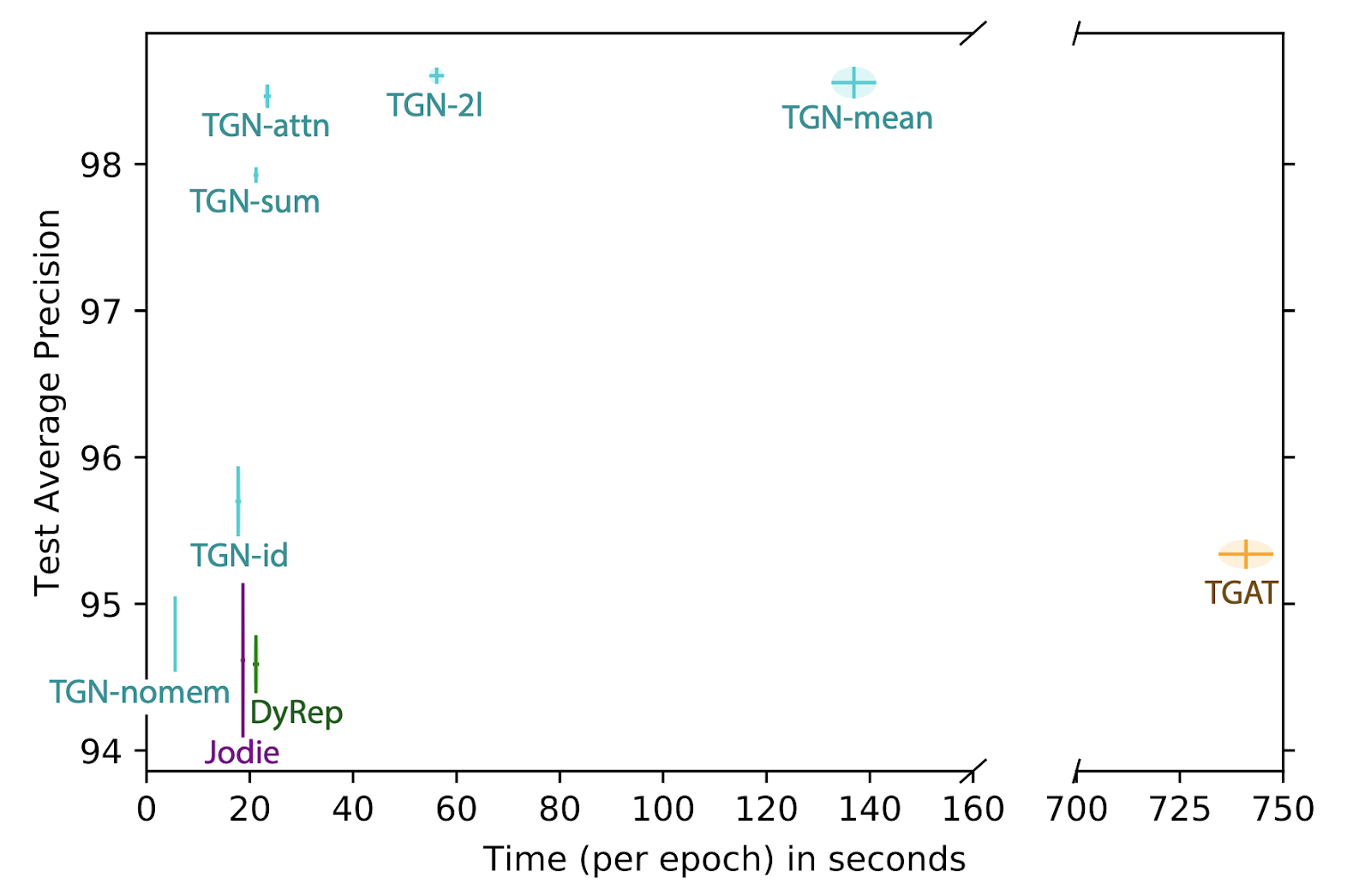
In experimental validation on various dynamic graphs, TGN significantly outperforms competing methods⁵ on the tasks of future edge prediction and dynamic node classification both in terms of accuracy and speed. One such dynamic graph is Wikipedia, where users and pages are nodes, and an interaction represents a user editing a page. An encoding of the edit text is used as interaction features. The task in this case is to predict which page a user will edit at a given time. We performed an extensive ablation study comparing different variants of TGN with baseline methods:

~The ablation study also shed light on the importance of different TGN modules, allowing us to make a few general conclusions. First, the memory is important: its absence leads to a large drop in performance⁶. Second, the use of the embedding module (as opposed to directly outputting the memory state) is important. Graph attention-based embedding appears to perform the best. Third, incorporating the memory allows us to only use one graph attention layer (which reduces the computation time by 3x), since the memory of 1-hop neighbors gives the model indirect access to 2-hop neighbors information.

For a more detailed explanation of the study, see our recently published paper. 

Conclusion

We consider learning on dynamic graphs an almost untouched research area, with numerous important and exciting applications and a significant potential impact. We believe that the TGN model is an important step towards advancing our ability to learn on dynamic graphs, consolidating and extending previous results. As this research field develops, better and bigger benchmarks will become essential. We are now working on creating new dynamic graph datasets and tasks as part of the Open Graph Benchmark. 

If you want to work on dynamic graphs, come join the flock!

¹ This scenario is usually referred to as “continuous-time dynamic graph”. For simplicity, here we consider only interaction events between pairs of nodes, represented as edges in the graph. Node insertions are considered as a special case of new edges when one of the endpoints is not presently in the graph. We do not consider node- or edge deletions, implying that the graph can only grow over time. Since there may be multiple edges between a pair of nodes, technically speaking, the object we have is a multigraph. 

² Multiple interactions can have the same timestamp, and the model predicts each one of them independently. Moreover, mini-batches are created by splitting the ordered list of events in contiguous chunks of a fixed size. 

³ For simplicity, we assume the graph to be undirected. In case of a directed graph, two distinct message functions, one for sources and one for destinations, would be needed.

⁴ J. Gilmer et al. Neural Message Passing for Quantum Chemistry (2017). arXiv:1704.01212. 

⁵ We also show that previous methods such as TGAT of D. Xu et al. Inductive representation learning on temporal graphs (2020), arXiv:2002.07962, Jodie of S. Kumar et al. Predicting dynamic embedding trajectory in temporal interaction networks (2019), arXiv:1908.01207 and DyRep of R. Trivedi et al. Representation Learning over Dynamic Graphs (2018), arXiv:1803.04051 can be obtained as particular configurations of TGN. For this reason, TGN appears to be the most general model for learning on dynamic graphs so far.

⁶ While the memory contains information about all past interactions of a node, the graph embedding module has access only to a sample of the temporal neighborhood (for computational reasons) and may therefore lack access to information critical for the task at hand.