Insights
Measuring the impact of Twitter network latency with CausalImpact
Twitter customers are significantly affected by network latency – the higher the latency, the less ideal the experience, as they cannot access Twitter content in a timely manner. To improve customer experience, we launched an experiment which aimed to lower latency by switching Twitter’s default edge to a faster public cloud edge in select countries. The switch should improve the baseline latency for all customers in these countries as public cloud edges have more geographical coverage in some regions. The experiment presented a unique challenge because due to network configuration, customers could not be randomly assigned to receive the treatment (i.e., faster app performance).
With a large customer base and network infrastructure, Twitter is in a unique position to develop and benefit from a framework to quantify the impact of an improvement in network latency. This article introduces the overall workflow and approach to quantify the causal impact of the experiment on revenue and customer engagement. While we measured only the impact on key topline metrics, the framework proposed is applicable to experiments with similar settings. We will also discuss how we adopted the CausalImpact package from Google, and which best practices we adhered to.
Inferring causality with Bayesian Structural Time Series (BSTS)
Causal impact of a treatment is the difference between the observed value of the response of the treated group and the counterfactual – the unobserved value that would have been obtained if the treated group was not treated. In an experiment where the treatment cannot be delivered randomly to customers, like the one presented here, only observed result data is available. This data could be contaminated by external shocks or bias. Modeling counterfactual and measuring causal effects are thus challenging. For our analysis, we adopted Google’s CausalImpact package which utilizes a BSTS model to infer causality in our network latency experiment.
As compared to more classical models, such as Difference-in-Difference and Synthetic Control, BSTS offers three advantages: (i) flexibility and modularity in accommodating different states such as seasonality, local trends and posterior variability; (ii) ability to infer impact and accommodate for decay and temporal variations; and (iii) means to model counterfactuals without the need for prior knowledge of external characteristics. The model adopts three main components to embed this: Kalman Filter, Spike-and-Slab Regression and Bayesian Averaging Model (stacking) with Gibbs Sampling. Read more on the main BSTS components and how the BSTS model can be used to infer causal impact on the provided links.
Constructing a robust analysis framework
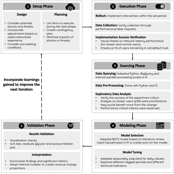
Conducting a causal impact analysis on the network latency experiment is challenging due to its setting. As discussed above, conducting a causal impact analysis on observed result data is not ideal because it could easily be affected by external shocks and biases. Having a robust framework to conduct the causal impact analysis is thus especially important because it will help us minimize potential shocks, produce robust results, and track new insights. In the next sections, we will present our adopted framework, and then discuss the steps and decisions that we made in each phase.
Emphasis on experiment design and setup
Having a good experiment design and setup is imperative as it determines the success of the experiment and the quality of the data collected. The scope of the experiment, along with metrics of interest, must be defined to avoid cherry picking data at a later stage.
Examples of points that we considered during the experiment design phase include:
- Scheduling: Avoid running experiments during holidays or observable seasonal patterns.
- Country Selection: Investigate which countries would be suitable for the experiment based on size of customer base, latency baseline, and percentage of customers directed towards the default host.
- Implementation Sequence and Acceleration: Consider the order in which the intervention should be implemented and investigate whether parallel implementation are possible – given that the counterfactual is created based on N - (# of target countries).
- Spillover Effect: Monitor the network latency on neighboring countries in case of spillover.
- Run Time: Consider implementing intervention for at least two months to accommodate for lagging effects on revenue and customer engagement metrics.
- Metrics Selection: Include all critical metrics – those that should remain stable throughout the experiment – and metrics of interest.
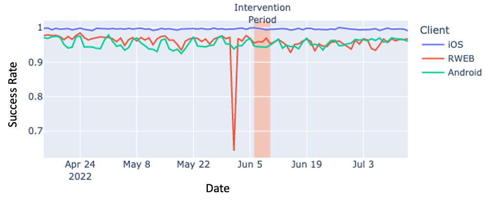
Validating the success of experiment rollout
Network latency performance metrics were used to validate the success of the intervention. Insignificant network latency changes would mean that intervention failed so no further analysis should be done. We selected and did visual checks on the slowest (95th percentile) and normal (50th percentile) to see if performance increased post-intervention. An example is shown in Figure 2. Close attention was given to the slowest customer group as they would have benefited most from improved performance.
To quantify performance, we selected content refresh time. It was chosen for three reasons:
- It is a common network request on a high impact surface area.
- The data is easily available.
- Our traffic map routing optimizes based on a similar metric.
In cases where visual checks were insufficient, we ran Difference-in-Difference (DiD) on performance with the target country. If no significance was found, we assumed that network latency did not improve.
Further checks on critical metrics such as request success rate, request volume and percentage of requests going through the default edge were also done to ensure they remained stable throughout the observation period. We proceeded with causal impact analysis with the BSTS model for the remaining metric groups after all of the validation steps were done.
Filtering the right metrics
Selecting key metrics that would allow us to quantify the causal impact of the experiment was a delicate process.
We selected four metric groups for the following reasons:
- Revenue: Exploration to identify whether performance has a direct impact on revenue.
- Customer State: Key leading indicators for future monetizable daily active customers and customer lifetime value.
- Customer Engagement: Exploration to identify whether performance has direct impact on engagement.
- Performance: Verification of rollout success and that the experiment did not impact customers’ experiences negatively.
Throughout the iterations, we added or removed metrics based on the following criteria:
- Data availability: Metrics which have lower sparsity and are readily available in well-maintained datasets are preferred.
- Sensitivity towards intervention: Metrics must be sensitive to react to the intervention and ideally with less time lag as external shocks — such as the Ukraine war — might occur and shorten the post intervention period.
- Suitability to key objectives: Metrics must be leading indicators for either revenue or customer engagement.
- Interpretability: Metrics and their impact must be easily explainable when they are found to be significant.
Observation period and challenges
We had more than one year of historical data to train the counterfactual model and roughly one month of post-intervention period (i.e., time after the new default edge was rolled out) data. We would have liked to have evaluated the data over a longer period of time, but the events in Ukraine would have had a significant exogenous influence on the results. For the more recent iterations, we had an even shorter period of time for some of the countries as network degradation occurred, as shown in Figure 5. The disruptions to the observation period emphasized the importance of selecting sensitive metrics and of evaluating our results for consistency. This is discussed in the next section.
Model tuning and evaluation
To build our model, we used covariates which are the metrics time series for other countries. For instance, if we are estimating the impact on variable_1 for South Africa, then we use the variable_1 time series for Japan, Brazil, Indonesia, etc. as covariates. For model selection, we ran a few different models with different prior.level.sd parameters and inclusion/exclusion of technical indicators, such as lagged covariates and moving averages covariates. We compared the performance of these models using cumulative absolute (1-step) error over the pre-intervention period during which there was no statistically significant impact. At the end, we chose the least complex model which included only lagged covariates to avoid overfitting. To further improve the BSTS model, adjustment towards the seasonality, dynamic regression, local linear trend, holiday and random walk parameters could also be considered.
Key learnings and takeaways
There are three key learnings we discovered when reiterating through our framework. We believe that these takeaways would be extremely valuable to anyone running similar experiments.
Results validation and robustness are crucial
Robustness and consistency of the inference are paramount as the consequence of an incorrect conjecture could cause the wrong business decisions to be made. We have implemented a few validation techniques such as the A/A test, residual and autocorrelation plots to validate our results. A case specific validation is also needed when the results obtained are inconclusive or inconsistent. For instance, we explored multiple time periods when degradation occurred in a country with a smaller customer base because our model could not produce a robust result. By undertaking the extra validation steps, we not only verified our results but also attained a better understanding of our model.
Zooming on counterintuitive results
We encountered some counterintuitive results during the later iterations whereby our selected metrics were significantly and negatively impacted.
A few further investigations that we often adopted to accommodate this issue includes:
- Adding more sensitive metrics (for example, those representing smaller subsets of customers).
- Checking for absolute impact to see if the customer base is too small.
- Running models with different periods.
- Checking for external shocks.
We found that these steps helped us either correct the results or at least shine light into potential explanations.
Grab opportunities from external shocks
External shocks could significantly affect rollout and results. When a contingency plan or workaround could not be implemented to contain the threat, these shocks presented an opportunity to gather new insights. When the host degradation occurred and network latency reverted back to its pre-intervention level for a country, we decided to probe whether inferring a causality for the period after degradation was possible. If our original hypothesis that an improvement in latency has a positive impact was correct, the hypothesis was that the degradation would have had a negative effect on revenue or engagement. The trial was not successful because the pre-intervention period was too short. Nonetheless, we learned that external shocks could be an opportunity to explore an impossible situation because we would have not been able to intentionally degrade latency for our users.
What’s next from here?
Although we were able to create a suitable framework to quantify the impact of network latency on revenue and customer engagement, there are a few considerations that could improve our study:
- Applying Cross Validation techniques during model selection.
- Comparing the performance of BSTS with other models such as Difference-in-Difference or Synthetic Control.
- Experimenting with subsets of customers for certain metrics.
- Finding the threshold of performance needed to make a significant impact on revenue and engagement for each country.
Acknowledgements
We’d like to thank our third author, Victor Ma, who is a Senior Data Scientist & Tech Lead for his contributions to this work and blog. The analysis would not have been possible without the engineers working on it: Irina Gracheva, Bernardo Rittmeyer as well as everyone on the Traffic Engineering and Platform Data Science teams who assisted on the project. We’d also like to thank individual editors and contributors who helped us write this article.